
This article summarizes my experience analyzing and predicting churn for a major US telecom provider. Since I worked in the telecom industry, subscriber service cancellations were called disconnects, and I will use churn, cancellations, and disconnects interchangeably.
Churn prediction model estimates the likelihood of a customer canceling their service during a specific future period of time. Churn prediction is used to understand churn drivers, evaluate retention programs, and calculate the lifetime value of the customer.
Predictive churn modeling is common in subscription businesses. Businesses that deal with individual transactions typically predict repurchases, i.e. calculate repurchase propensity scores for their customers. Repurchase propensity modeling is similar to churn modeling, except for the data preparation step, which is different due to transactional data structure.
Exploratory Analysis and Feature Engineering
The first step to creating a churn prediction model is exploratory analysis. I wrote a very detailed post on how to perform this analysis here.
The exploratory analysis shows which variables have a relationship with churn, and such input factors add value to the model. It will also show whether the relationships between continuous input variables and churn rate are linear.
In the case of non-linear relationships, you either have to use a model that accommodates for non-linearity, like a decision tree model, or you can transform your input variables into dummy variables corresponding to high and low churn. In machine learning, dummy variable transformation is called one-hot encoding.
For example, when analyzing churn for a telecom company, I looked at the relationship between churn and tenure and split the tenure variable into dummy variables corresponding to high and low churn periods. This made it possible to use a linear model such as logistic regression for churn prediction.
Categorical Data Preparation
To be used effectively in the model, categorical variables also need to be turned into dummy variables (one-hot encoding), which are a series of 1 or 0 flags.
For example, if you have a variable that has three values and indicates that a customer is “under a contract”, is “out of contract”, or has “never been in contract”, then you can use two variables to encode whether the customer is in contract (1=yes, 0=no), out of contract (1=yes, 0=no), but you don’t have to create the third, since everyone who is neither in contract nor out of contract (0 and 0) is going to be in the “never been in contract” category.
Temporal Data and Data Leaks (Information Feedback Loops)
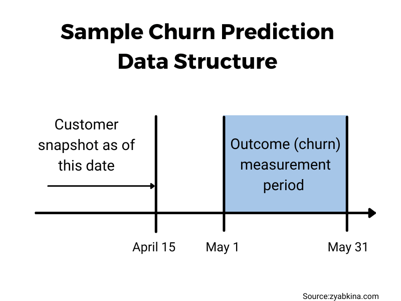
The data used in predictive churn modeling is temporal data. That means that every variable is valid on a specific date. As the timeframe shifts, the data for the same subscriber may change.
For example, let’s consider a variable “number of service tickets created within a 90-day period”. As of January 1st, subscriber X had 2 service tickets created in the 90 prior to the snapshot date. If subscriber X creates another ticket on January 2nd and the oldest ticket is still no longer than 90 days out, then as of January 3rd, subscriber X would have 3 service tickets created within 90 days.
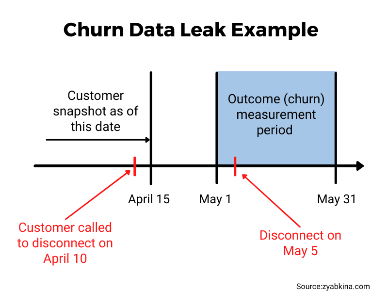
When creating a predictive model, it is very important for the input validity periods to not overlap with the output (churn) validity period. Otherwise, churn artifacts may appear in your input data, turning your model into a self-fulfilling prophecy.
To choose the right input and output periods, you need to understand how the model will be used. One of the most meaningful questions to ask is when the prediction needs to be updated relative to the start of the outcome period.
For example, if you need to provide a churn score for every active customer on the 15th of every month, and this churn score should predict customer churn during the next calendar month, all of your input variables need to be valid as of the 15th of the prior month or earlier.
Information about upcoming churn can sip into your data in other ways. For example, if customers schedule their cancellations up to 30 days in advance by calling your cancellation phone number, you should not include calls to this phone line unless they are over 30 days before the start of the churn measurement period. If you don’t, you are predicting that subscribers would cancel after they had already called to cancel, which is a self-fulfilling prophecy.
Churn Predictors
Independent variables, predictors, regressors, or features are input variables that show the status of the subscriber before the churn prediction period. This data can come from two general sources: internal data about the subscriber that is generated during the relationship, and external data, which is either collected by the company or bought from a vendor.
This is the data commonly used as churn predictors in the telecom industry. Your list will be different, but the idea is to find variables correlated with customer churn.
Data from internal sources:
- Product or service the customer is subscribing to. If the customers are able to subscribe to multiple services, then segmenting the customers by major product groups or bundles makes sense. For example, cable video service plus internet service is a popular bundle.
- Tenure. Customer tenure is the length of time since the beginning of the customer relationship. It is an extremely important variable in churn analysis.
- Changes to the product or service prior to the snapshot date. These are usually bellwethers of more changes to come and thus correlate to future churn levels.
- Channel the customer connected through. Different types of customers self-select into different channels.
- Service outages, tickets, and workorders. Customers like their services to work well. Issues with the service can result in an increased level of churn.
- Product usage. How and how much your customers use your product. Please note that there could be privacy restrictions on which usage data you are able to analyze.
- Payment history. Being late on the bill is a big indicator of future churn.
Data from external sources:
- Demographics. The staples of demographic data are customer gender, age, education, and income. However, for many subscription services, variables related to transitivity or propensity to move are also important. These are variables such as the time at residence and homeowner status.
- Competition. Many residential subscription services are limited to a particular geography. Understanding which competitor services are available to the customer is an important factor.
Churn Data
Your model’s dependent variable or label is whether the customer churns in the output period of time. However, defining churn can be tricky. For example, when I worked in telecom, I analyzed subscriber disconnects by reason, and since the dynamic and input factors were different by different types of disconnects, we had to create separate models.
The type of churn model you need to create may also be defined by how the model is going to be used. If the goal of the model is to facilitate a timely payment program, then predicting non-pay cancellations makes the most sense.
In businesses that use annual billing, a churn prediction model is equivalent to a subscription renewal model. In this case, the subscription renewal is an easy event to record, but the analyst needs to pay attention when the model needs to be run. For example, predicting subscription renewal 11 months ahead may help estimate customer lifetime value. Predicting renewal 60 days in advance may help evaluate retention programs.
In short, make sure your output variable makes sense for the task at hand.
Types of Predictive Churn Models
There are several types of models that are being used to predict churn. All of them have outputs/predictions that range from 0 to 1, to reflect the outcome at the end of the prediction period (1=churned, 0=active). The most common model is logistic regression.
Logistic regression
This is the most basic model. If you don’t know where to start, start here. The model is similar to multiple regression, except it uses a sigmoid function to transform the output and bind it to (0 to 1) range.
If you are not sure about whether certain attributes or variables should be included in the model, you can add regularization (Lasso, Ridge), which will drive coefficients of insignificant variables to zero.
Logistic regression is a simple, but powerful modeling method, and I can’t recommend it highly enough.
Random Forests and Decision Tree Based Models:
If you are new to predictive modeling and know how to use R or Python, then random forests are a good place to start.
Random forests are a decision tree-based ensemble method that has two excellent qualities: they are hard to overfit, and they handle non-linear variables well. The downside is opacity, as it’s hard to see which variables impact the outcome and by how much.
Support Vector Machine (SVM)
SVMs are machine learning models that have become popular recently because of their excellent performance in challenging competition cases. It works by creating an optimized boundary between outcomes.
There are several types of models that fall under SVMs, which means that the analyst has to choose the method and its hyperparameters for the model to make the most sense. My recommendation is to have a seasoned modeler implement SVMs.
Neural Networks (RNN, LSTM)
The simplest neural network that predicts a binary outcome using one node and a sigmoid output is logistic regression. If you want to go further, increasing the number of layers and nodes you run a serious risk of overfitting.
But don’t fret, deep learning approaches like Long Short Term Memory (LSTM) models might be able to help. If you are running longitudinal analysis using input variables with a fairly long history (think IoT sensor data), you can feed them into a special kind of Recurrent Neural Network model called LSTM. This model feeds your data through layers and combines the effects of history into a prediction.
If you are a novice in machine learning, I would recommend sticking to simpler methods, though.
Bayesian (Hierarchical Bayes Models)
These models usually predict the time to disconnect and are widely used in lifetime value (LTV) estimation. Bayesian modes presume that the expected time to disconnect for each customer follows gamma distribution, parameters of which may, in turn, come from another distribution.
The Bayesian model uses a stepwise fitting method, such as Markov Chain Monte Carlo to estimate the parameters of these distributions.
If you decide to go this route, get someone who has done Bayes modeling (successfully, i.e. it converged) before. These can be tricky.
Training, Validation, and Test Samples
When creating predictive models our goal is to make them accurate. The challenge comes with some models that can be overfitted, i.e. are too complicated for the data that we have, and thus try to accommodate every point in our dataset (aka remember them) instead of teasing out general principles of how the data points are distributed.
To prevent overfitting and test the accuracy, modelers use test samples. The observation dataset is split into training and testing samples randomly, and only the training data is used for fitting the model. The test sample (usually 10%-20%) of the dataset is used to estimate model accuracy on the data that the model has not “seen” before.
A validation sample is similar to the test sample, but it is used for hyperparameter estimation. Hyperparameters are foundational settings of advanced models (random forests, SVMs, LSTMs) that define the structure of the model itself. Several models with different settings are trained first, and the validation sample is used to choose the best combination of hyperparameters. Then, the best model’s accuracy is estimated using the test sample.
Conclusion
Creating a good churn propensity model takes domain knowledge, data familiarity, and modeling proficiency. You may have to go through multiple iterations of introducing new data and changing the type of the model before achieving a good result.
What constitutes a good result is relative, but researchers found that most churn models achieve what is called 3-4 times “lift”, which is the ratio between the actual churn rate of the top decile (top 10%) of customers predicted by your churn model and average churn rate. For example, if your top decile churned at 8% in the predicted period, and the average for the whole predicted population was 2%, then you achieved (8% / 2%) = 4 times lift.
Before you embark on the churn prediction exercise you need to understand how you are going to be able to use the results. If you are planning to target those most likely to churn, you are likely to find the result underwhelming and off the mark. However, there are multiple ways to use effectively use churn propensity scores, so read my next article that explains how to get value from predictive models.